Strategy Update:

1) The latest run result as followed:

Last PL: 2910213 
Biggest drawDown: -498050.6 
Total buy(times): 15 
Total sell(times): 5 
Max Margin: 4434984 
max buy position: 22 
max sell position: -20 
start money: 5e+06 
Annual return: 0.4590242 
Volatility: 
Max Max Drawdown(Ratio): 0.08078893

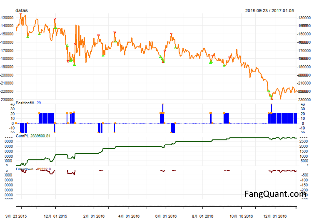
2) Strategy chart:

We observed that spread continued to widen between SSE50 and A50, probably due to tightness in China money market and the expectation of RMB devaluation, which made investors hesitate to long SSE50, so the SSE50 price showed increasing weakness against A50.

The newest hedging ratio between SSE50 and A50 is 1:13, instead of 1:14 in our report in October 2016.

As the picture above:

The yellow lines is the trend of difference (SSE50*300– 13*A50*USDCNY);

The green points mean SSE50 is under-valued, and we long SSE50,short A50.

The red points mean that SSE50 is over-valued, and we short SSE50, long A50.

The blue line below present the changing of the positions we build due to the strategy.( up one point means we long the spread one time, down one point means we short the spread one time)

The dark green and red lines below present the return and the maximum drawback of the strategy respectively.

The dates of buying and selling signal are listed below:

> rownames(as.data.frame(datas[datas$buy>0]))
 [1] "2015-11-05" "2015-12-18" "2015-12-24" "2015-12-25" "2015-12-30" "2016-05-24"
 [7] "2016-05-26" "2016-05-27" "2016-05-30" "2016-08-12" "2016-08-15" "2016-09-02"
[13] "2016-11-22" "2016-11-24" "2016-11-25"

To be more specific, the buying signals after October 2016 are listed below:

> buys[buys>as.Date('2016-10-01')]
[1] "2016-11-22" "2016-11-24" "2016-11-25"

3) Strategy review:

We adopted the widely used mean-reversion strategy to generate signal for the SSE50-A50 Spread Trading system.

The daily residual from fitting A50 on SSE50, named “e”, is treated as “stock price”, to calculate the moving average. A large deviation from the average meant there’s trading opportunity.

We regressed A50 on SSE50 with the first 50 daily close prices, with the R code below, and get the first e.

for(i in (L+1):num_all){  
  lm1<-lm(y_all[1:(i-1)]~x_all[1:(i-1)]) 
  e_all[i]<-y_all[i]-lm1$coefficients[[2]]*x_all[i]-lm1$coefficients[[1]]
}

For the moving average of e we used 30-day mean, as in R code below:

mas[i]<-mean(past_prices) sigmas[i]<-sd(past_prices) 

Lastly, the newest e is compared to moving average of e and calculated the deviation.

daily_sigma[i] = (current_price - mas[i]) / sigmas[i]  

The times of deviation over sigma is also calculated as a measure of winning probability, as R code below.

for(sig in minp:(maxp-w-1)){
  wls<-my_data[my_data$pvs>=sig&my_data$pvs<(sig+w),2]
  ratio=sum(wls=="win")/length(wls)
  if(length(wls)/total >= least_percentage){
    if(best_ratio<ratio){
      best_ratio<-ratio
      lower<-sig
      uper<-sig+w
    }
  }
}

4) The graph showed the residual e of A50 fitting with SSE50 and upper and lower bounds of sigmas.

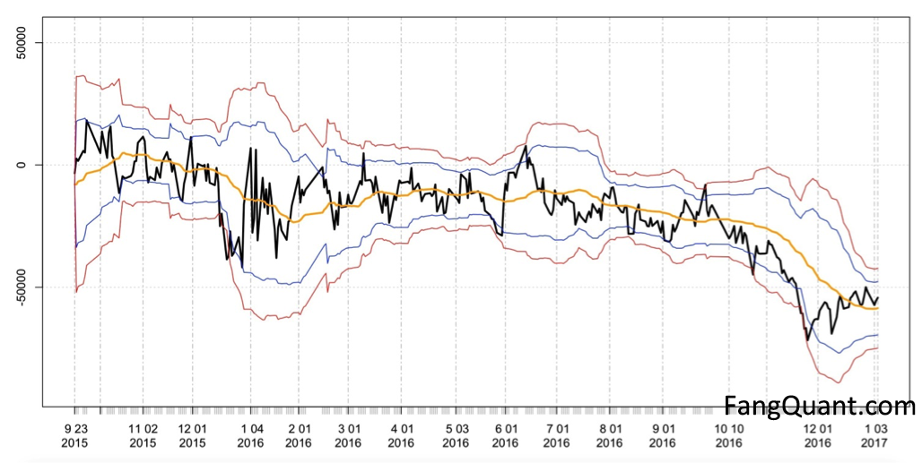
The black line is the trend of daily residual e;

The yellow line is the trend of daily average MA;

The red and blue lines are the trend of upper and lower bounds which calculated according to the deviation ρ and volatility σ.