Steps:
Ⅰ.estimate the model coefficients
Ⅱ.build a strategy with a stable expected return

Ⅰ.Estimate the model coefficients
We set the data range from 2015/4/16—2016/8/26 to run the regression.

1. The independent variables for CSI300 and SSE50 are named as x and y respectively. The dependable variable A50 is named as z. Each index is multiplied by the contract multiplier and converted into Chinese Yuan.
First of all, we calculated the correlation between each two of the indexes as following:

> cor(x,y)
[1] 0.9850738
> cor(x,z)
[1] 0.9364365

The correlation is high between each pair of the three.

2. And we run the ordinary least square (OLS) linear regression in R:

> lm1<-lm(z~x+y)
> lm1

Call:
lm(formula = z ~ x + y)
Coefficients:
(Intercept) x y 
17959.0566 -0.0223 0.1027 

The result showed some defects:
1) The intercept is an oversized number.
2) The coefficient for x, CSI300, is negative. And there’s collinearity between x and y.

3. The graph below showed obvious collinearity between CSI300 and SSE50:

4. Process with ridge regression:
We applied regularization method to set a limit for the intercept. And run the ridge regression to process the data with collinearity.
With lm.ridge()function, we acquired 151 lambdas and selected the lambda with Generalized Cross Validation (GCV) when lambdaGCV is at minimum.

The ridge trace is plotted with minimum lambdaGCV as below:

> ridge.sol<-lm.ridge(z~x+y,lambda=seq(0,150,length=151),model=TRUE)
> names(ridge.sol)
[1] "coef" "scales" "Inter" "lambda" "ym" "xm" "GCV" "kHKB" "kLW" 
> ridge.sol$lambda[which.min(ridge.sol$GCV)]
[1] 0
> ridge.sol$coef[which.min(ridge.sol$GCV)]
[1] -300.4365
> par(mfrow=c(1,2))
> matplot(ridge.sol$lambda,t(ridge.sol$coef),xlab=expression(lambda),ylab="Cofficients",type="l",lty=1:20)
> abline(v=ridge.sol$lambda[which.min(ridge.sol$GCV)])

And also with the graph of lambda and GCV:
> plot(ridge.sol$lambda,ridge.sol$GCV,type="l",xlab=expression(lambda),ylab=expression(beta))
> abline(v=ridge.sol$lambda[which.min(ridge.sol$GCV)])

The ridge trace is stabilized in a narrow range when lambda rose above 50.

Firstly GCV is calculated for lambda at 0 as below:

> ridge.sol<-lm.ridge(z~x+y,lambda=0,model=TRUE)
> ridge.sol$GCV
0 
4341.567
&gt; models = lm.ridge(rt$A50~rt$CSI300+rt$SSE50,lambda=seq(0,150,len=150))
rt$CSI300 rt$SSE50
0.000000 17485.04 -0.001586841 0.07127925
1.006711 17804.23 0.002810185 0.06422905
2.013423 18044.22 0.005794676 0.05941096
116.778523 25822.98 0.017710798 0.03060350
117.785235 25875.29 0.017693995 0.03055534
118.791946 25927.45 0.017677140 0.03050745
119.798658 25979.47 0.017660236 0.03045983
120.805369 26031.36 0.017643286 0.03041248
147.986577 27382.69 0.017174862 0.02921970
148.993289 27430.98 0.017157316 0.02917829
150.000000 27479.14 0.017139766 0.02913706

The coefficient for x and y are still too small, as the contract value of A50 is much smaller compared to CSI300 and SSE50, as below:

> mean(rt$CSI300)
[1] 1070110
> mean(rt$SSE50)
[1] 712673.9
> mean(rt$A50)
[1] 66585.81

We run regression with Lambda ranged from 0-150 and estimated x at 0.018 and y at 0.03;
The model is 18CSI300+30SSE50-1000A50=D
Or 9CSI300+15SSE50-500A50=D/2
That is to say, long 9 lots CSI300 and 15 lots SSE50,short 500 lots A50.

Ⅱ.Trading Strategy:
1. The residual and N-day mean graphs are as below: (N=10,20,50,60)

And we showed expected P&L with different N and T as below:

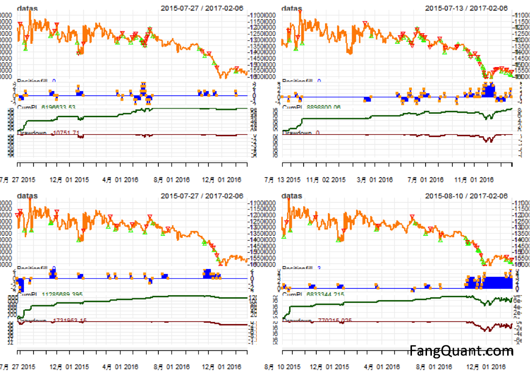
The parameters are:

N =10, T =60 (upper left):
Last PL: 6196634
Biggest drawDown: -968984.4
Total buy(times): 15
Total sell(times): 8
Max Margin: 11210945
max buy position: 2
max sell position: -2
start money: 1.4e+07
Annual return: 0.294293
Max Max Drawdown(Ratio): 0.05400559

N =10, T =50 (upper right):
Last PL: 8898800
Biggest drawDown: -3145767
Total buy(times): 26
Total sell(times): 11
Max Margin: 24738480
max buy position: 4
max sell position: -2
start money: 2.8e+07
Annual return: 0.2037271
Max Max Drawdown(Ratio): 0.08820586

N =20, T =50 (bottom left):
Last PL: 11285689
Biggest drawDown: -1731953
Total buy(times): 12
Total sell(times): 5
Max Margin: 20037091
max buy position: 2
max sell position: -3
start money: 2.5e+07
Annual return: 0.3033787
Max Max Drawdown(Ratio): 0.05588578

N =20, T =60 (bottom right):
Last PL: 6833344
Biggest drawDown: -3373134
Total buy(times): 20
Total sell(times): 2
Max Margin: 30399882
max buy position: 5
max sell position: -1
start money: 3.8e+07
Annual return: 0.1238463
Max Max Drawdown(Ratio): 0.07396646

After comparison of the parameters above, we picked N=10&T=60 and N=20&T=50 as parameters for the trading strategy.

Append:

The collinearity is checked with lasso (least absolute shrinkage and selection operator) regression:

> A<-as.matrix(rt[,3:4])
> B<-as.matrix(rt[,2])
> laa=lars(A,B,type="lar")

Call:
lars(x = A, y = B, type = "lar")
R-squared: 0.979 
Sequence of LAR moves:
SSE50 CSI300
Var 2 1
Step 1 2

The lasso method ranked SSE50 before CSI300 as expected.

> summary(laa)
LARS/LAR
Call: lars(x = A, y = B, type = "lar")
Df Rss Cp
0 1 2.3467e+10 15702.7815
1 2 4.9092e+08 1.5306
2 3 4.9015e+08 3.0000

The Mallows's Cp is calculated to access the collinearity. The smaller the Cp the better the fit. So by this criteria, it’s more proper to hedge A50 with SSE50 only.

copyright by FangQuant.com