Summary
In this work, we observe yield differences of indices and whether they could be predicted by time series generated by themselves. We find that it possible to get significantly positive payoff by trying our strategy on the time series of yield difference between SSE50 and CSI500 over a 50-month period but not for SSE50 and A50.

1. Indices introduction
The SSE50 index is based on the scientific and objective method to select the 50 most representative stocks in the Shanghai securities market, which are the largest and abundant in liquidity. The intention of the index is to comprehensively reflect the overall situation by a group of leading enterprises with the most market influence in the Shanghai securities market. The SSE50 index has been officially released since January 2, 2004. The goal is to set up an investment index that is active, large and can be a base for derivative instruments.
The FTSE China A50 Index(A50) is a real-time tradable index comprising the 50 largest A Share companies. The index offers the optimal balance between representativeness and tradability for China A Share market with its indicators, including performance, liquidity, volatility, industry distribution and market representativeness, are at the leading level of the market.

CSI Small-cap 500 index (CSI500) is one of the index developed by the China Securities Index Co. The stock in the sample space is made up of 500 remaining largest stocks in the total A shares after dropping the top 300 stocks in the total market value or the components of CSI 300 index. The index comprehensively reflects performance of a group of small and medium market capitalization companies in A shares.

Table 1: Summary of the 3 indices.

2. Indices yield difference.

We observe yield difference of indices, we mainly focus on R(SSE50)-R(CSI500) and R(SSE50)-R(A50) and try to find whether such difference is predictable or there is such strategy that making superior performance.

In this work, we focus on monthly difference, we choose a time period of 100 months up to 2018/6/29

Graph 1: Monthly R(SSE50)-R(CSI500) Time Series

Graph 2: Monthly R(SSE50)-R(A50) Time Series

3. Candidate factors.

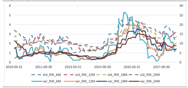
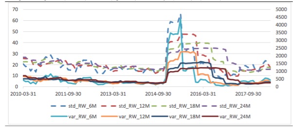
In this work, there several factors we employed to check whether they can be used to predict the difference. Here the factors we considered are generated from the yield difference time series themselves.
In detail, the factors we evaluated include lag 1,2,3,4,5 and 6 yield difference, annualized sample standard deviation and annualized sample variance of previous 6, 12,18and 24 periods.

Graph 3: Sample Std (left axis) and Var (right axis) of Monthly R(SSE50)-R(A50) Time Series

Graph 4: Sample Std (left axis) and Var (right axis) of Monthly R(SSE50)-R(CSI500) Time Series

4. Regression analysis
In this work, our regression is done in such a way that we use every combination of these 14 factors to regress the monthly yield difference series (so, there would be C141+ C142+...+ C1414 =16383 combinations). When conduct regression, yield difference at time T is corresponded to factors at time (T-1) to observe the if there is predictive power.
We would divide the 100-month period into 2 equal parts to check whether the potential predictive ability is stable.
Over the later 50-month period we fund that there are several statistically significant (under 5% significance level) relationships (127 significant relations for R(SSE50)-R(CSI500) and 101 for R(SSE50)-R(A50). And the minimum p-values for R(SSE50)-R(CSI500) and R(SSE50)-R(A50) are 0.0119 and 0.0157 respectively (in Appendix). However, over the earlier 50-month period, no significant linear relationship of prediction is observed in these 16383 regressions. The p-values of F are at least 0.2 and 0.07 for these 2 series respectively.
Therefore, for factors we considered, there is no stable linear relationship to make prediction.

5. Potential Strategy
The relationship between the yield difference and factors is not stable over long time, as the environment of the market keeps changing. However, it may be effective during a limited period if relations are so significant. That is, if we find some predictive relationship by observing data over period from T1 to T2, then this relation may exist over period T2 to T2+dT.

So, the strategy is, find the best predictive relation (the one with the lowest p-value of F) during T1=(T-1-P) to T2=(T-1), if its p-value of F is below 0.05, then use this relationship to predict the indices yield difference, dR, at T (making out of ample prediction), then trade by the predicted result (long one short the other). If the best predictive relation’s p-value of F is above 0.05, do nothing.

Graph 5: Strategy logics

We set P=50 Month, if our prediction is correct (the signal of predicted dR is the same as the actual dR), earn |dR(T)|, otherwise loose |dR(T)|. We earn 0 if there is no action.
Under such strategy the cumulative profit for time series of R(SSE50)-R(CSI500) is 31.98%, for time series of R(SSE50)-R(A50) is -0.06%. Obviously, the payoff for applying on time series of R(SSE50)-R(A50) is quite low and can be even lower with transaction expense.

Table 2: Strategy back test result for applying time series of R(SSE50)-R(CSI500)

Table 3: Strategy back test result for applying time series of R(SSE50)-R(A50)

6. Result Discussion
There are several points we would like to mention.
Our strategy actually refreshes prediction model at each month. A benefit of this is that it would accept and adapt market environment change. That is, a prediction relationship may change over time, our strategy only assumes the past relationship would persist 1 period ahead. In fact, in each case (table 2 or 3), we can observe that the predictive relation change over time (Best Potential Combination to Predict changed over time).
However, actually, for the relation with lowest p-value of F, the explanation power is not high as R^2 is usually low. So, our strategy would give only limited superior performance and frequently make prediction error. Then, more factors should be considered to deal with this. In future work, we would consider other factors related to fundamental prospects or macroeconomic factors.

In our strategy, the calculation workload is high. With inputs of 14 factors, 100-month data, 50-month horizon to find relation, we totally do 16383502=1638300 regression calculations to work out table 2 and table 3 and this need computer to run several hours. Thus, if more factors are considered, the number of combination would dramatically rise then the time to work out back test would be very long. So, at each time, we can only jointly consider limited number of factors (about 12).

Appendix

Table 4: 5%-level Significant Combinations for R(SSE50)-R(CSI500) series over the later 50-month period.

Table 5: 5%-level Significant Combinations for R(SSE50)-R(A50) series over the later 50-month period.

# setup
R2_limit=0
f_pv_limit=0.05
D_Period = 50
FInput_Y=pd.read_excel(filename,'Y')
FInput_X=pd.read_excel(filename,'X')

def Reg_Selection(f_pv_limit,R2_limit,FInput_X,FInput_Y):
    Count_Comb=0
    Count_Selected=0
    Num_N=len(FInput_X.index)
    Num_X=len(FInput_X.columns)
    Min_f_p=1
    for Num_Var in range(1, Num_X+1):
        U=list(combinations(FInput_X,Num_Var))
        for Detail_Comb in U:
            Comb_X={}
            for list_i in Detail_Comb:
                se=FInput_X[[list_i]]
                d_se={'%s'%(list_i):se.transpose().get_values()[0]} 
                Comb_X.update(d_se)
            F_Comb_X=pd.DataFrame(Comb_X) 
            F_Comb_X.index=FInput_Y.index 
            X_S=sm.add_constant(F_Comb_X)
            est=sm.OLS(FInput_Y ,X_S).fit()
            Count_Comb+=1
            if est.f_pvalue<Min_f_p:
                Max_adj_R2=est.rsquared_adj 
                Min_f_p_Comb=Detail_Comb
                Min_f_p=est.f_pvalue
                Min_f_est=est
            if (est.f_pvalue<=f_pv_limit) and (est.rsquared>=R2_limit):
                Count_Selected+=1
    return (Min_f_est, Min_f_p_Comb)
def Masive_Reg_Selection_Back_Test(f_pv_limit, D_Period):
    Num_N=len(FInput_X.index)
    L_pre=[]
    Comb=[]
    Real=[]
    Correct=[]
    Gain=[]
    PV_F=[]
    for i in range(1, Num_N-D_Period+1):
        Sel_X=FInput_X.iloc[i:i+D_Period,:]
        Sel_Y=FInput_Y.iloc[i:i+D_Period,:]
        Reg_sel=Reg_Selection(f_pv_limit,R2_limit,Sel_X,Sel_Y)
        EST_i=Reg_sel[0]
        Comb_i=Reg_sel[1]
        if (EST_i.f_pvalue < f_pv_limit):
            Num_in_var = EST_i.df_model
            min_p_f_reg='%.6lf\t'%(EST_i.params[0]) 
            preidc_i_1=EST_i.params[0]
            j=0
            while j<Num_in_var:
                min_p_f_reg = min_p_f_reg + '%.6lf\t' % (EST_i.params[j + 1])
                j+=1
            c_v=0
            for list_i in Comb_i: 
                c_v+=1
                k=0
                for mark in FInput_X.axes[1]:
                    if mark==list_i: 
                        list_loc=k
                        preidc_i_1 = preidc_i_1 + EST_i.params[c_v] * FInput_X.get_values()[i - 1][list_loc]
                        break
                    else:
                        k+=1
            print(i,Comb_i,EST_i.f_pvalue,'\n%s\npredic=%.6lf\n\n'%(min_p_f_reg,preidc_i_1))
            L_pre = L_pre + [preidc_i_1]
            Comb = Comb + [Comb_i]
            if np.sign(FInput_Y.get_values()[i - 1][0]) == np.sign(preidc_i_1):
                c = 1
            else:
                c = -1
        else:
            print(i, 'No Act')
            L_pre=L_pre+[0]
            Comb = Comb + ['No Act']
            c = 0
        Correct = Correct + [c]
        Real = Real + [FInput_Y.get_values()[i - 1][0]]
        Gain = Gain + [abs(FInput_Y.get_values()[i - 1][0]) * c]
        PV_F = PV_F + ['%.6lf' % (EST_i.f_pvalue)]
    dic_pre = {'Real': Real, 'Predic': L_pre, 'Comb': Comb, 'P-value of F': PV_F, 'Correct': Correct, 'Gain': Gain}
    W1=pd.ExcelWriter('%s'%(sq_2)) 
    dic_pre = pd.DataFrame(dic_pre)
    dic_pre.to_excel(W1, 'Predict')
    W1.save()
Masive_Reg_Selection_Back_Test(f_pv_limit,D_Period) 

copyright by fangquant.com